This post will take us through the process of building, from scratch, an image classification model using stochastic gradient descent (SGD).
Ok, great - building a model from scratch. But what should we model?
Since the 90’s the default data set for testing out image classification models has been MNIST - a collection of 70,000 greyscale handwritten digits. For the most part it’s a great data set, the major drawback (in my opinion) - it’s incredibly boring (maybe if they used my handwriting it would be more exciting?).

[Above] A visualization of some of the MNIST data taken from Wikipedia.
Thankfully, a team of researchers put together Fashion MNIST, a fun collection of greyscale fashion images.
Similarly to MNIST there are 10 classes, but each is a type of clothing.
| Label | Description |
|---|---|
| 0 | T-shirt/top |
| 1 | Trouser |
| 2 | Pullover |
| 3 | Dress |
| 4 | Coat |
| 5 | Sandal |
| 6 | Shirt |
| 7 | Sneaker |
| 8 | Bag |
| 9 | Ankle boot |
Examples of these data below (from the project Github page - each class takes three rows):
![]()
Well, I may be fashion challenged - but the fashion MNIST is much more entertaining - let’s use that for this experiment!
Project Goal
In this lil’ post, we will train a binary classifier to determine if a given image is a sneaker or a shirt.
Getting Started
To start, let’s load the important libraries and explore our data.
from fastai.vision.all import *
import numpy as np
import torchvision
import torchvision.transforms as transforms
%matplotlib inline
import matplotlib.pyplot as plt
matplotlib.rc('image', cmap='Greys')
Getting the data
Pytorch conveniently has some shortcuts for us to download the Fashion MNIST data, which we’ll take advantage of here. And, like most curated ML data sets, there are pre-defined training and test sets.
trainset = torchvision.datasets.FashionMNIST(root = "./notebooks/storage", train = True, download = True, transform = transforms.ToTensor())
testset = torchvision.datasets.FashionMNIST(root = "./notebooks/storage", train = False, download = True, transform = transforms.ToTensor())
Ok, what does this data look like?
type(trainset)
torchvision.datasets.mnist.FashionMNIST
print(trainset.data.shape, trainset.targets.shape)
torch.Size([60000, 28, 28]) torch.Size([60000])
The data sets contain primarily a .data and .targets attributes. .data is a rank 3 tensor of shape [60000, 28, 28]. In reality, this tensor is 60,000 images of size 28px by 28px. As expected, .targets is a rank 1 tensor of shape 60,000 - indicating the class of each image in .data.
Since in this project we are only interested in two types of clothing, let’s grab our sneakers (7) and shirts (6).
trainset_x = trainset.data[(trainset.targets == 6) | (trainset.targets == 7)]
trainset_y = trainset.targets[(trainset.targets == 6) | (trainset.targets == 7)]
Next, we can split our trainset into training and validation sets (remember - the test set was already broken out for us).
d_length = trainset_x.shape[0]
# 10% can go to validation
validation_ix = random.sample(range(0, d_length),round(d_length*0.1))
train_ix = np.setdiff1d(range(0, d_length),validation_ix)
trainX = trainset_x[train_ix]
trainy  = trainset_y[train_ix]
validX = trainset_x[validation_ix]
validy = trainset_y[validation_ix]
print(f'training set size: {trainy.shape[0]}\nvalidation set size: {validy.shape[0]}')
training set size: 10800
validation set size: 1200
We can take a peak with FastAI’s handy show_image function to see what this data looks like.
random_ix = [0,100,2]
show_image(trainX[random_ix[0]]);
show_image(trainX[random_ix[1]]);
show_image(trainX[random_ix[2]])
print(['shirt' if i.item() == 6 else 'sneaker' for i in trainy[random_ix]])
['sneaker', 'sneaker', 'shirt']


Ok, those pictures are pretty cool, but what does that data actually look like? Surely the data has some sort of numerical representation?
Well, we already know each image is a 28x28 tensor. Each element of that matrix is an integer representing its darkness (0 is white, 255 is black, everything in the middle is grey).
Let’s take a quick look at a pandas heatmap representation of the data. We can see the 28X28 grid, the values ranging from 0 to 255.
df = pd.DataFrame(trainX[0])
df.style.set_properties(**{'font-size':'6pt'}).background_gradient('Greys')
| 0 | 1 | 2 | 3 | 4 | 5 | 6 | 7 | 8 | 9 | 10 | 11 | 12 | 13 | 14 | 15 | 16 | 17 | 18 | 19 | 20 | 21 | 22 | 23 | 24 | 25 | 26 | 27 | |
|---|---|---|---|---|---|---|---|---|---|---|---|---|---|---|---|---|---|---|---|---|---|---|---|---|---|---|---|---|
| 0 | 0 | 0 | 0 | 0 | 0 | 0 | 0 | 0 | 0 | 0 | 0 | 0 | 0 | 0 | 0 | 0 | 0 | 0 | 0 | 0 | 0 | 0 | 0 | 0 | 0 | 0 | 0 | 0 |
| 1 | 0 | 0 | 0 | 0 | 0 | 0 | 0 | 0 | 0 | 0 | 0 | 0 | 0 | 0 | 0 | 0 | 0 | 0 | 0 | 0 | 0 | 0 | 0 | 0 | 0 | 0 | 0 | 0 |
| 2 | 0 | 0 | 0 | 0 | 0 | 0 | 0 | 0 | 0 | 0 | 0 | 0 | 0 | 0 | 0 | 0 | 0 | 0 | 0 | 0 | 0 | 0 | 0 | 0 | 0 | 0 | 0 | 0 |
| 3 | 0 | 0 | 0 | 0 | 0 | 0 | 0 | 0 | 0 | 0 | 0 | 0 | 0 | 0 | 0 | 0 | 0 | 0 | 0 | 0 | 0 | 0 | 0 | 0 | 0 | 0 | 0 | 0 |
| 4 | 0 | 0 | 0 | 0 | 0 | 0 | 0 | 0 | 0 | 0 | 0 | 0 | 0 | 0 | 0 | 0 | 0 | 0 | 0 | 0 | 0 | 0 | 0 | 0 | 0 | 0 | 0 | 0 |
| 5 | 0 | 0 | 0 | 0 | 0 | 0 | 0 | 0 | 0 | 0 | 0 | 0 | 0 | 0 | 0 | 0 | 0 | 0 | 0 | 0 | 0 | 0 | 0 | 0 | 0 | 0 | 0 | 0 |
| 6 | 0 | 0 | 0 | 0 | 0 | 0 | 0 | 0 | 0 | 0 | 0 | 0 | 0 | 0 | 0 | 0 | 0 | 0 | 0 | 0 | 0 | 0 | 0 | 0 | 0 | 0 | 0 | 0 |
| 7 | 0 | 0 | 0 | 0 | 0 | 0 | 0 | 0 | 0 | 0 | 0 | 0 | 0 | 0 | 0 | 0 | 0 | 0 | 0 | 0 | 0 | 0 | 0 | 0 | 0 | 0 | 0 | 0 |
| 8 | 0 | 0 | 0 | 0 | 0 | 0 | 0 | 0 | 0 | 1 | 1 | 0 | 3 | 1 | 0 | 4 | 0 | 0 | 0 | 2 | 0 | 0 | 0 | 0 | 5 | 1 | 0 | 0 |
| 9 | 0 | 0 | 0 | 0 | 0 | 0 | 0 | 0 | 0 | 0 | 0 | 0 | 4 | 0 | 0 | 0 | 0 | 0 | 106 | 229 | 0 | 0 | 0 | 0 | 0 | 0 | 0 | 0 |
| 10 | 0 | 0 | 0 | 0 | 0 | 0 | 0 | 0 | 0 | 0 | 1 | 0 | 0 | 0 | 0 | 90 | 138 | 223 | 214 | 209 | 167 | 0 | 0 | 0 | 6 | 124 | 0 | 0 |
| 11 | 0 | 0 | 0 | 0 | 0 | 0 | 0 | 0 | 1 | 0 | 0 | 0 | 37 | 122 | 179 | 249 | 214 | 195 | 181 | 213 | 241 | 0 | 0 | 0 | 94 | 179 | 0 | 0 |
| 12 | 0 | 0 | 0 | 2 | 0 | 6 | 0 | 0 | 0 | 0 | 16 | 149 | 236 | 226 | 201 | 195 | 200 | 204 | 155 | 209 | 116 | 0 | 22 | 109 | 251 | 35 | 51 | 0 |
| 13 | 0 | 0 | 1 | 3 | 0 | 0 | 0 | 0 | 67 | 150 | 240 | 221 | 194 | 190 | 204 | 214 | 205 | 195 | 207 | 185 | 206 | 233 | 224 | 179 | 2 | 10 | 22 | 0 |
| 14 | 0 | 0 | 0 | 0 | 0 | 0 | 110 | 214 | 237 | 209 | 196 | 192 | 215 | 215 | 213 | 213 | 207 | 193 | 186 | 199 | 206 | 175 | 0 | 0 | 124 | 230 | 200 | 36 |
| 15 | 0 | 50 | 119 | 158 | 166 | 192 | 204 | 198 | 187 | 202 | 203 | 211 | 214 | 204 | 209 | 210 | 204 | 197 | 191 | 190 | 191 | 229 | 230 | 242 | 214 | 193 | 203 | 137 |
| 16 | 108 | 190 | 199 | 200 | 194 | 199 | 194 | 195 | 199 | 200 | 189 | 187 | 191 | 189 | 197 | 198 | 205 | 200 | 200 | 208 | 213 | 215 | 212 | 213 | 209 | 202 | 216 | 137 |
| 17 | 15 | 55 | 114 | 157 | 188 | 207 | 216 | 220 | 217 | 219 | 221 | 242 | 240 | 243 | 249 | 253 | 255 | 255 | 243 | 232 | 226 | 222 | 221 | 213 | 215 | 198 | 209 | 62 |
| 18 | 16 | 11 | 0 | 0 | 7 | 40 | 76 | 108 | 134 | 142 | 143 | 145 | 143 | 123 | 111 | 92 | 76 | 61 | 45 | 35 | 25 | 25 | 31 | 32 | 32 | 12 | 1 | 0 |
| 19 | 0 | 11 | 25 | 26 | 26 | 22 | 12 | 20 | 15 | 15 | 18 | 17 | 19 | 27 | 30 | 36 | 41 | 49 | 57 | 66 | 79 | 84 | 79 | 83 | 93 | 80 | 75 | 45 |
| 20 | 0 | 0 | 0 | 0 | 0 | 9 | 14 | 17 | 27 | 34 | 39 | 39 | 42 | 44 | 41 | 41 | 43 | 48 | 43 | 30 | 31 | 35 | 40 | 37 | 40 | 37 | 26 | 0 |
| 21 | 0 | 0 | 0 | 0 | 0 | 0 | 0 | 0 | 0 | 0 | 0 | 0 | 0 | 0 | 0 | 0 | 0 | 0 | 0 | 0 | 0 | 0 | 0 | 0 | 0 | 0 | 0 | 0 |
| 22 | 0 | 0 | 0 | 0 | 0 | 0 | 0 | 0 | 0 | 0 | 0 | 0 | 0 | 0 | 0 | 0 | 0 | 0 | 0 | 0 | 0 | 0 | 0 | 0 | 0 | 0 | 0 | 0 |
| 23 | 0 | 0 | 0 | 0 | 0 | 0 | 0 | 0 | 0 | 0 | 0 | 0 | 0 | 0 | 0 | 0 | 0 | 0 | 0 | 0 | 0 | 0 | 0 | 0 | 0 | 0 | 0 | 0 |
| 24 | 0 | 0 | 0 | 0 | 0 | 0 | 0 | 0 | 0 | 0 | 0 | 0 | 0 | 0 | 0 | 0 | 0 | 0 | 0 | 0 | 0 | 0 | 0 | 0 | 0 | 0 | 0 | 0 |
| 25 | 0 | 0 | 0 | 0 | 0 | 0 | 0 | 0 | 0 | 0 | 0 | 0 | 0 | 0 | 0 | 0 | 0 | 0 | 0 | 0 | 0 | 0 | 0 | 0 | 0 | 0 | 0 | 0 |
| 26 | 0 | 0 | 0 | 0 | 0 | 0 | 0 | 0 | 0 | 0 | 0 | 0 | 0 | 0 | 0 | 0 | 0 | 0 | 0 | 0 | 0 | 0 | 0 | 0 | 0 | 0 | 0 | 0 |
| 27 | 0 | 0 | 0 | 0 | 0 | 0 | 0 | 0 | 0 | 0 | 0 | 0 | 0 | 0 | 0 | 0 | 0 | 0 | 0 | 0 | 0 | 0 | 0 | 0 | 0 | 0 | 0 | 0 |
I really love the pandas heatmap representation of the data to really understand the structure!
Interestingly, it is harder for me to recognize the image as a shoe zoomed in though - a true Monet.
show_image(trainX[random_ix[0]])
<AxesSubplot:>

Now that we are familiar with our data, let’s see if we can train a model to classify these images.
Approach - Linear Regression
Here we will train a linear model to determine if an image is a sneaker (7) or a shirt (6). Linear regressions are usually used to predict continuous outcomes and have the form
$$\hat{y{i} = \beta{0} + \beta{1} x{i,1} + … + \beta{p} x{i,p}$$
or, in matrix algebra
\(\textbf{y} = X \bf{\beta} + \bf{\epsilon}\)
Since we are not predicting a continuous variable (ie. dollars spent on popcorn, GDP, net worth of celebrities, etc.) but instead estimating class assignment, we can map these predictions to probabilities (i.e. values in [0,1]) with the sigmoid function.
$$S(x) = \frac{1}{1+e^{-x}}$$
If that function looks weird, that’s ok! Let’s just plot it to make sure it’s doing what we think it’s doing.
def sigmoid_function(x):
    return(1/(1+np.exp(-x)))
x=np.arange(-6,6,0.1)
plt.plot(x,sigmoid_function(x))
[<matplotlib.lines.Line2D at 0x7efec02362b0>]
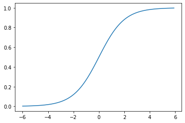
Yup! Looks like \(s(x)\) is bounded by 0 and 1.
Fitting our Logistic Regression with Stocastic Gradient Descent (SGD)
So we have a model (logistic regression) - great! Now - how do we fit it? - Stocastic Gradient Descent (SGD).
For those who may not be familiar, SGD is an iterative approach to model fitting that is very popular in deep/machine learning. The basic premise of SGD is we make predictions using our model and subsets of our training data (minibatchs), we determine how ‘good’ our model did by evaluating the loss for each batch, and slowly move model parameters to minimize the loss.
Specifically, SGD involves the following steps:
a.) initialize (or generate) random weights - This would be our beta coefficients above ($\beta_1$ through $\beta_k$ we will refer to as our weights, $\beta_0$ as our bias).
b.) for each batch of data, use our model and weights to predict each image’s class
c.) compute how the loss (how good or bad our model was)
d.) compute the gradient* for each weight
e.) update our weights using the gradients
f.) repeat steps b-e until we have a good model
Step 0 - Let’s get our data in the correct formats
In order to run these experiments we will need to transform our training features to be a single vector of size 784 (that’s just 28 times 28) instead of the current 28X28 tensor. We will also transform our target to 1 when the image is a sneaker and 0 when a shoe.
# for the training set
train_x = trainX.view(-1,28*28).float()
train_y = torch.where(trainy==torch.tensor(6),torch.tensor(1),torch.tensor(0)).unsqueeze(1)
train_x.shape,train_y.shape
(torch.Size([10800, 784]), torch.Size([10800, 1]))
# for the validation set
valid_x = validX.view(-1, 28*28).float()
valid_y = torch.where(validy==torch.tensor(6),torch.tensor(1),torch.tensor(0)).unsqueeze(1)
valid_x.shape,valid_y.shape
(torch.Size([1200, 784]), torch.Size([1200, 1]))
a.) initialize (or generate) random weights
In order to start SGD we need to have some random parameters initialized.
def initialize_params(size):
    return (torch.randn(size)).requires_grad_()
Now we can initialize our weights and bias
weights = initialize_params((28*28,1))
bias = initialize_params(1)
weights.shape,bias.shape
(torch.Size([784, 1]), torch.Size([1]))
b.) for each batch of data, use our model and weights to predict each image’s class
Next, lets define our model.
We have: - our features: $X$ (1x784) - our weights: $\beta$ (784x1) - our bias: $\epsilon$ (1x1)
$$\hat{P(x_i = \text{Shirt})} = S(X \bf{\beta} + \bf{\epsilon})$$
where $S(x)$ is the sigmoid function defined as
$S(x) = \frac{1}{1+e^{-z}}$
def logistic_regression(x):
    # x is our pixel values
    # weights are our beta coefficients
    # bias is our bias term
    return (x@weights + bias).sigmoid()
c.) compute how the loss (how good or bad our model was)
Now, we actually have enough infrastructure (parameters and a model which uses the parameters) to make some (bad) ‘predictions’ using our logistic_regression model.
As my 3rd grade teacher would say, let’s make mistakes! (miss frizzle)
model_predictions = logistic_regression(train_x)
model_predictions[0:3]
tensor([[1.],
        [0.],
        [1.]], grad_fn=<SliceBackward>)
Drum roll please!
And our overall accuracy is:
corrects = (model_predictions>0.0) == train_y
corrects.float().mean().item()
0.6226851940155029
So the accuracy here isn’t great, but hey what can we expect, we are essentially randomly determining the image’s class.
Now that we have the ability to make predictions with our model we need to assess the performance in a very granular way. Accuracy is a metric that tells us how we are performing in a very human interpretable way, but we can actually change the weights and have the same accuracy. Imagine 2 models trying to assess if an image of a Yorkie is a dog or a cat. Model A may say that the image is a dog with 57% confidence while model B may think the image is a dog with 99% confidence. Assuming we have a decision boundary of 50%, both models would be ‘correct’ but clearly model B deserves more credit.
A good loss function will capture these differences resulting in different ‘loss’ for the same ‘accuracy’. The simplest loss function is the mean absolute error (sometimes known as L1 loss). So to keep things simple we will use that.
def l1_loss(predictions, targets):
    predictions = predictions.sigmoid()
    return (targets-predictions).abs().mean()
d.) compute the gradient for each weight
For SGD we will feed our model a series of random slices of data, compute the gradeint for each parameter (weights), updating them accordingly in order to minimize the models loss for each iteration of the entire data set (epoch).
I’m going to use fast.ai’s DataLoader class here to construct this iterator for both the training and validation sets.
dataset = list(zip(train_x,train_y))
dl = DataLoader(dataset, batch_size=270,shuffle=True)
valid_dset = list(zip(valid_x,valid_y))
valid_dl = DataLoader(valid_dset, batch_size=240,shuffle=True)
We can look at the first iteration of the dataloader which shows us that we have 270 rows of size 784 (28X28)
xb,yb = first(dl)
xb.shape,yb.shape
(torch.Size([270, 784]), torch.Size([270, 1]))
Quick aside: How SGD works.
Without getting too much into the weeds here, SGD works by - making predictions using the given weights - computing how ‘off’ those predictions were by calculating a loss - computing the gradient (derivative) of the loss - moving the weights to minimize the loss - new_weights = old_weights - weights_derivative*constant
The derivative** is computed automatically for us by Pytorch using the .backward() attribute. The inner workings of this ‘autograd’ out of the scope of this post.
The ‘constant’ we are referring to here is also known as the ‘learning rate’ in the literature.
We can define a function that computes the model parameter gradients (derivative) with respect to our loss function.
def calc_grad(x, y, model_fn, loss_fn=l1_loss):
    preds = model_fn(x)
    loss = loss_fn(preds, y)
    loss.backward()
Great! Once we have the gradient we can use them to update the parameters in order to minimize the loss.
e.) update our weights using the gradients
def update_parameters(parameters,lr):
    for param in parameters:
        param.data -= param.grad*lr
        param.grad.zero_()
f.) repeat steps b-e until we have a good model
Now we can put these pieces together.
For each batch within an epoch, we need to compute the loss of our model, determine the parameters’ gradient (calc_grad) and update the parameters accordingly (steps b-e).
We can define our train epoch function below to do this for us.
def train_epoch(model_fn,lr,params,training_data,valid_data):
    for x,y in training_data:
        calc_grad(x,y,model_fn,loss_fn = l1_loss)
        update_parameters(params,lr)
While not technically necessary to generate our model, it would be helpful to print out how well our model is performing as we train it. We can define an accuracy function to print the accuracy of our model against some some held out data.
def accuracy(model_fn,x,y):
    preds = (model_fn(x)>0.5)
    acc = (preds == y).float().mean()
    print(f'accuracy: {round(acc.item()*100,2)}%')
Let’s run our model!
So we can now use our initialize_params function to initialize our parameters (weights, bias), and our train_epoch function to fit the model for several epochs.
torch.manual_seed(50)
weights = initialize_params((28*28,1))
bias = initialize_params(1)
epochs = 20
lr = 0.1
for i in range(epochs):
    train_epoch(model_fn = logistic_regression,
               lr=lr,
               params = (weights,bias),
               training_data=dl,
               valid_data=valid_dl)
    accuracy(model_fn = logistic_regression,
                  x=valid_x,
                  y=valid_y)
accuracy: 46.92%
accuracy: 49.83%
accuracy: 54.67%
accuracy: 60.92%
accuracy: 72.0%
accuracy: 80.25%
accuracy: 83.83%
accuracy: 89.33%
accuracy: 91.83%
accuracy: 92.67%
accuracy: 93.33%
accuracy: 93.67%
accuracy: 93.83%
accuracy: 94.5%
accuracy: 94.5%
accuracy: 94.42%
accuracy: 94.75%
accuracy: 95.25%
accuracy: 95.25%
accuracy: 95.42%
Wow! After 20 epochs (that took about 3 seconds to run) we are at over 97% accuracy in our out of sample validation set.
Now, let’s see how we perform on our test set.
accuracy(model_fn = logistic_regression,
                  x=train_x,
                  y=train_y)
accuracy: 94.84%
Voilà! Over 95% - not bad!
We now have an image classifier built from scratch! In building this tool, we also implemented SGD and found our performance to be pretty great for a few lines of code! Hopefully, you can take the information in this post and build your own classifier or extend this one!
There were a few aspects of SGD and image classification that we glanced over, as well as a lot of tricks modern image recognition models use to improve speed and performance. But the core of these modern models is exactly what we just saw!
Other Notes:
* The gradient here is the slope of the loss with respect to the model parameters. If we can compute the slope of the loss, we can move our parameters where the slope is negative to reduce our loss and yield a better model.
Example: we know loss(x,p) has derivative -2 at current p. Therefore increating the value of p a small amount (\(p_2=p-(-2) * \epsilon\) ) should lower the value of loss(x,\(p_2\)).
** We can’t have SGD without computing the gradient. The Pytorch autograd is what computes the gradients (AKA derivatives) for us. We totally took this crucial part for granted in this post, but it’s a really important and impressive piece of technology that drives modern deep learning.