Since food is such an important aspect of life and public health, I thought it would be exciting to look at food trends over time. Obviously food choices drive public health, but I figured that trends were just this - trends, preferences that may change over time. While a bit broad, I narrowed down ‘food trends’ to be interest in Chipotle Mexican Grill - a fan favorite - over time. Since I don’t readily have any real Chipotle sales data, I decided to make my own - well, kinda.
Using Google trends, we can look at “how often a particular search-term is entered relative to the total search-volume across various regions of the world”, and this, if we squint, might be close enough to sales data that we can use it as a rough proxy - with a few exceptions. Obviously sometimes interest in a company means something quite different than sales - just think of all of the equifax searches that have occurred in the past few weeks.
JAGS or STAN
Since this is a Bayesian approach, I felt that there were two options available: use JAGS or STAN, I went with JAGS for no particular reason other than being slightly more familiar with the syntax and feeling that it may be a better beginner language for those without much Bayesian computing experience. Those without JAGS experience are more than welcome to follow along, but might want to check out this to learn more!
Step 1: Getting data (yes, guac please)
First we will grab some chipotle data using the really nice gtrendsR R package. There are a few parameters to pay attention to here, so don’t be afraid to look them up! Of particular interest to us is the keyword (chipotle), the region (USA), time span (note: Google rewards shorter time spans with higher resolution data - good to keep in mind; we will be using 5 years), and category (Food & Drink). Here we are searching for just the name of the restaurant.
library(gtrendsR)
chipotle_gtrends <- gtrends(keyword = "chipotle",
                geo = "US",
                time = "all",
                category = 71)
gtrends returns a lot of information, maybe even too much for us:
str(chipotle_gtrends)## List of 6
## $ interest_over_time:'data.frame': 166 obs. of 6 variables:
## ..$ date : Date[1:166], format: "2004-01-01" ...
## ..$ hits : int [1:166] 11 12 12 11 12 14 15 14 13 13 ...
## ..$ keyword : chr [1:166] "chipotle" "chipotle" "chipotle" "chipotle" ...
## ..$ geo : chr [1:166] "US" "US" "US" "US" ...
## ..$ gprop : chr [1:166] "web" "web" "web" "web" ...
## ..$ category: int [1:166] 71 71 71 71 71 71 71 71 71 71 ...
## $ interest_by_region:'data.frame': 51 obs. of 5 variables:
## ..$ location: chr [1:51] "Ohio" "District of Columbia" "Maryland" "Minnesota" ...
## ..$ hits : int [1:51] 100 91 87 80 66 65 63 61 53 52 ...
## ..$ keyword : chr [1:51] "chipotle" "chipotle" "chipotle" "chipotle" ...
## ..$ geo : chr [1:51] "US" "US" "US" "US" ...
## ..$ gprop : chr [1:51] "web" "web" "web" "web" ...
## $ interest_by_dma :'data.frame': 206 obs. of 5 variables:
## ..$ location: chr [1:206] "Columbus OH" "Cincinnati OH" "Cleveland-Akron (Canton) OH" "Minneapolis-St. Paul MN" ...
## ..$ hits : int [1:206] 100 99 97 76 73 73 71 68 65 64 ...
## ..$ keyword : chr [1:206] "chipotle" "chipotle" "chipotle" "chipotle" ...
## ..$ geo : chr [1:206] "US" "US" "US" "US" ...
## ..$ gprop : chr [1:206] "web" "web" "web" "web" ...
## $ interest_by_city :'data.frame': 50 obs. of 5 variables:
## ..$ location: chr [1:50] "Columbus" "Overland Park" "Alexandria" "Cincinnati" ...
## ..$ hits : int [1:50] 100 95 93 88 80 76 73 72 71 71 ...
## ..$ keyword : chr [1:50] "chipotle" "chipotle" "chipotle" "chipotle" ...
## ..$ geo : chr [1:50] "US" "US" "US" "US" ...
## ..$ gprop : chr [1:50] "web" "web" "web" "web" ...
## $ related_topics :'data.frame': 16 obs. of 6 variables:
## ..$ subject : chr [1:16] "100" "10" "5" "0" ...
## ..$ related_topics: chr [1:16] "top" "top" "top" "top" ...
## ..$ value : chr [1:16] "Chipotle Mexican Grill" "Chipotle" "Burrito" "Adobo" ...
## ..$ geo : chr [1:16] "US" "US" "US" "US" ...
## ..$ keyword : chr [1:16] "chipotle" "chipotle" "chipotle" "chipotle" ...
## ..$ category : int [1:16] 71 71 71 71 71 71 71 71 71 71 ...
## $ related_queries :'data.frame': 50 obs. of 6 variables:
## ..$ subject : chr [1:50] "100" "40" "40" "35" ...
## ..$ related_queries: chr [1:50] "top" "top" "top" "top" ...
## ..$ value : chr [1:50] "chipotle menu" "chipotle recipe" "chipotle near me" "nutrition chipotle" ...
## ..$ geo : chr [1:50] "US" "US" "US" "US" ...
## ..$ keyword : chr [1:50] "chipotle" "chipotle" "chipotle" "chipotle" ...
## ..$ category : int [1:50] 71 71 71 71 71 71 71 71 71 71 ...
## - attr(*, "class")= chr [1:2] "gtrends" "list"So we can go ahead an remove what we want: total interest and time (although a more in-depth analysis could definitely use the extra information) which is contained as a data.frame in the interest_over_time portion of the list which we will extract.
chip_dat <- chipotle_gtrends$interest_over_timeLet’s see what we have here:
plot(chip_dat$date, chip_dat$hits, type = "l", lwd = 4,
     main = "Google trends: Chipotle Resturants",
     ylab = "Hits", xlab = "Date",  cex.lab = 1.3,
     cex.main = 1.4, cex.axis = 1.3)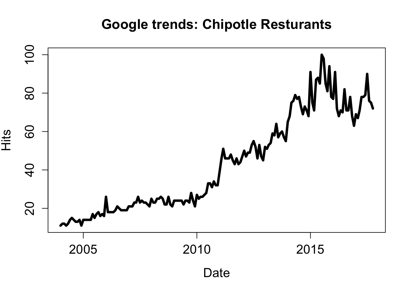
Whoa! Looks good!
As always, when conducting an analysis, we want to make sure any assumptions are sufficiently met. With some time series analyses, data must be stationary, defined as mean, variance, and autocorrelation remaining constant over time. A quick way of (usually) achieving this is by examining differences.
library(dplyr)
hits_dif <- diff(chip_dat$hits)
date_dif <- chip_dat$date[-1]
plot(date_dif, hits_dif, type = "l", lwd = 3,
main = "Google trends: Chipotle Resturants - First Diff",
ylab = "Hits (diff)", xlab = "Date ", cex.lab = 1.3,
cex.main = 1.4, cex.axis = 1.3)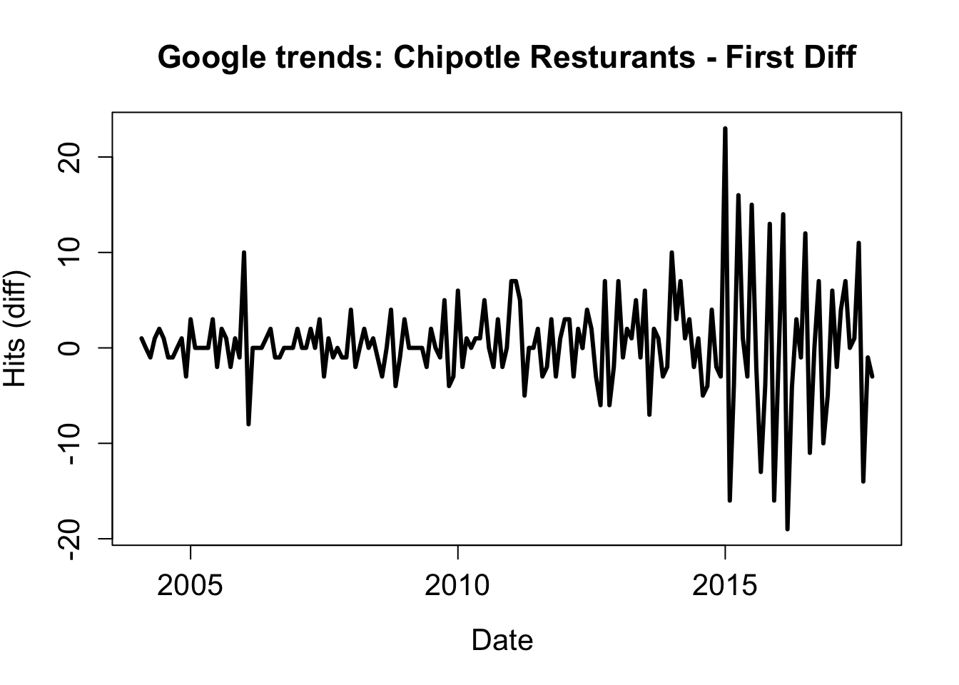
So we notice that the mean hovers around zero in the first difference which is good, although the variance is clearly not stable. That is ‘OK-enough’ for this small example, but the problem could be possibly be alleviated by taking the second difference, or using another method of standardization, each of which has its own set of issues.
Intercept Model
Now that we have our differenced data lets look at a very simple model - the intercept model - by which the first difference is modeled as a function of only a constant term (\(\mu\)) and an error term (\(\epsilon\))
\(y_t = \mu + \epsilon_t\)
Note: Perhaps now it is clear why we need stationary data, the intercept only model could not capture a moving mean, but rather only a constant mean with constant variance.
Lets load some important packages we will be using
library(R2jags)     # for using JAGS in R
library(jagstools)  # Some additional JAGS tools
library(knitr)      # I love the kable function
library(coda)       #
Now, lets define our model (\(y_t = \mu + \epsilon_t\)) in JAGS.
model.1 <- function() {
        # priors on parameters

        # mean ~ normal: mean = 0, sd = 1/sqrt(0.01)
        mu ~ dnorm(0, 0.01);

        # tau ~ inverse gamma: alpha, beta = 0.001
        tau.obs ~ dgamma(0.001,0.001);

        # sd is treated as derived parameter
        sd.obs <- 1/sqrt(tau.obs);

        for(i in 1:N) {
                Y[i] ~ dnorm(mu, tau.obs);
        }
}
Now we can define our data, parameters, and run the model.
set.seed(100)
N = length(hits_dif)

jags.data = list("Y"=hits_dif,"N"=N) # named list of inputs

jags.params=c("sd.obs","mu") # parameters to be monitored

mod_lm_intercept = jags(jags.data, parameters.to.save=jags.params,
                        model.file=model.1, n.chains = 3, n.burnin=5000,
                        n.thin=1, n.iter=10000, DIC=TRUE)
## module glm loaded## Compiling model graph
## Resolving undeclared variables
## Allocating nodes
## Graph information:
## Observed stochastic nodes: 165
## Unobserved stochastic nodes: 2
## Total graph size: 176
##
## Initializing modelGreat! Now lets investigate some of the results. Primarily, what values are plausible for \(\mu\) and what sort of variability we have.
par(mfrow = c(2,1))

hist(mod_lm_intercept$BUGSoutput$sims.matrix[,2],
     40,col="grey",
     xlab="Mean",
     main="")

hist(mod_lm_intercept$BUGSoutput$sims.matrix[,3],
     40,col="grey",xlab=expression(sigma[obs]),main="")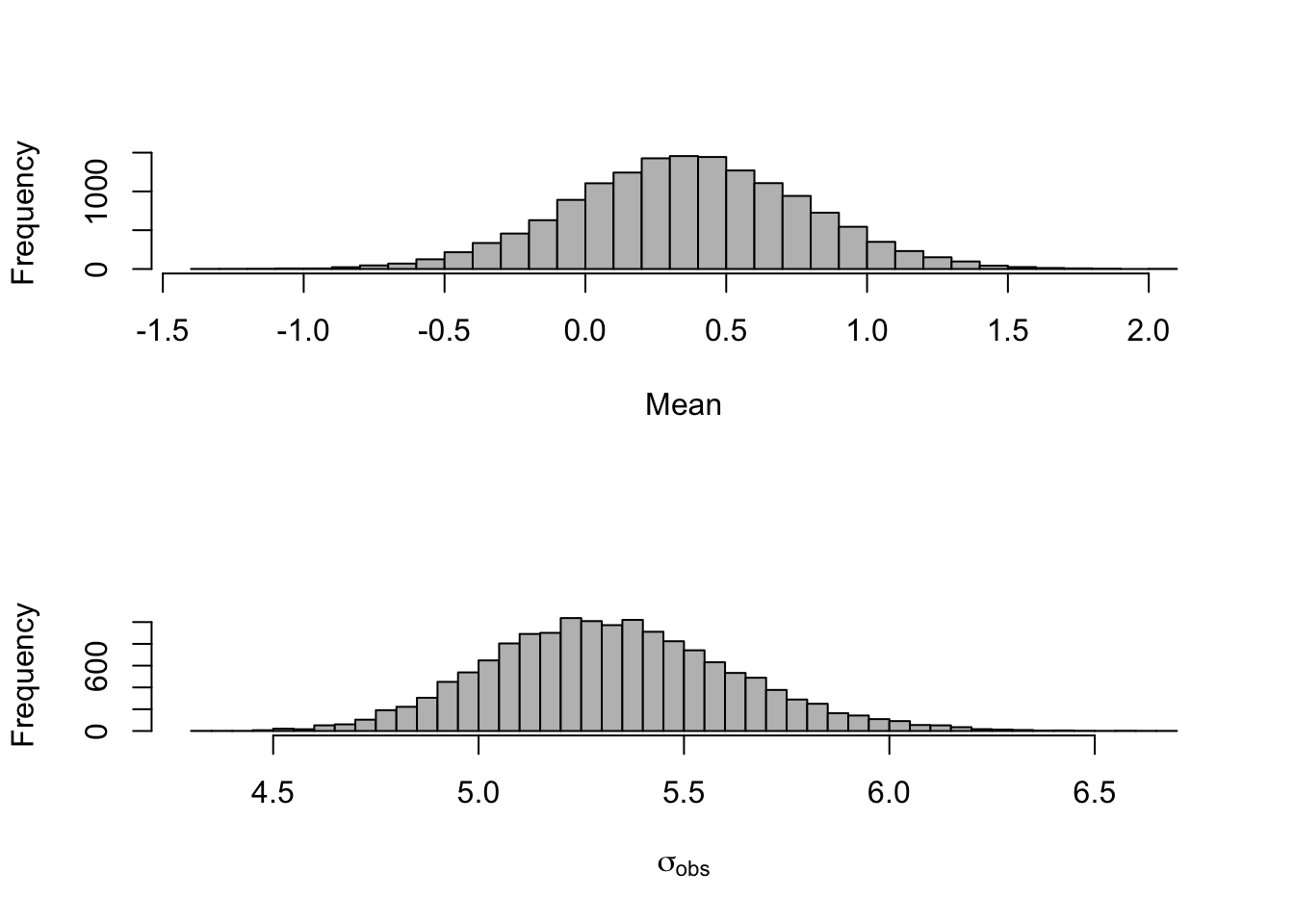
Below is a function I stole from the Bayesian Methods II course at the JHUSPH which allows us to produce some informative plots about our MCMC. Without getting too detailed, these plots can illustrate plausible values of our parameters as well as provide some insight into whether or not our model has converged.
createMcmcList = function(jagsmodel){
        McmcArray = as.array(jagsmodel$BUGSoutput$sims.array)
        McmcList = vector("list",length=dim(McmcArray)[2])
        for(i in 1:length(McmcList)) McmcList[[i]] = as.mcmc(McmcArray[,i,])
        McmcList = mcmc.list(McmcList)
        return(McmcList)
}
myList = createMcmcList(mod_lm_intercept)
plot(myList[[1]])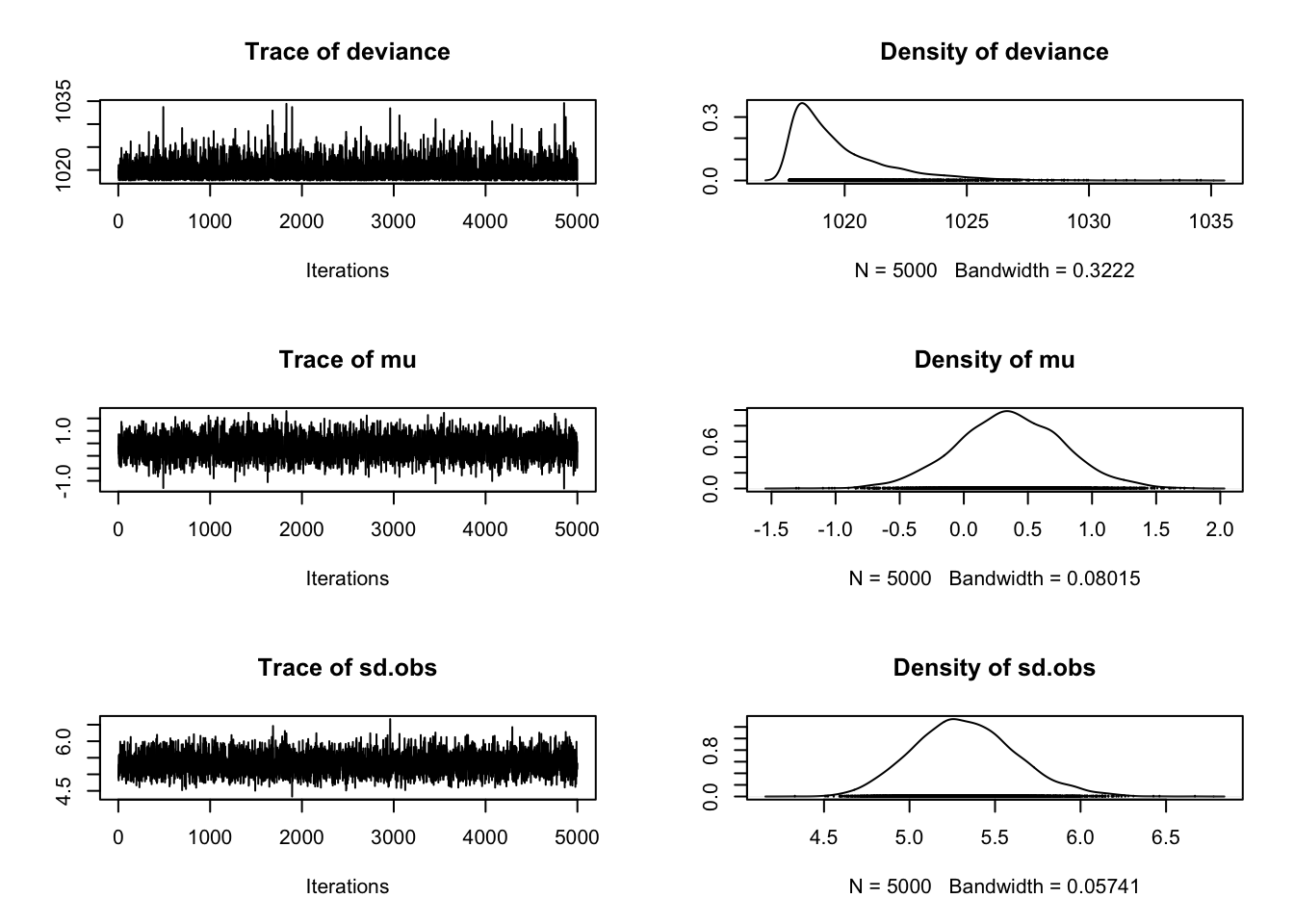
We wont spend too much time on these results, because this extremely simple model may be too difficult to draw informative inference from. So, we will examine a slightly more complex model next.
Autocorelated Error Model
Here we will try a similar model, but allow for non-independence of errors. More specifically, we allow the deviation from the mean \(\mu\) to be a function of the previous deviation \(e_{t-1}\) scaled by a parameter to be estimated, \(\phi\).
\(E(y_t) = \mu + \phi * e_{t-1}\)
We can enter this into jags as so:
ar.model <- function(){
                # priors on parameters
                # very diffuse
                mu ~ dnorm(0, 0.01)
                tau.obs ~ dgamma(0.001,0.001)
                sd.obs <- 1/sqrt(tau.obs)
                phi ~ dunif(-1,1) # autocorrelation must be between -1,1
                tau.cor <- tau.obs * (1-phi*phi) # Var = sigma2 * (1-rho^2)
                epsilon[1] <- Y[1] - mu
                predY[1] <- mu # initial value

                # skipping first value (it doesnt have a difference)
                for(i in 2:N) {
                        predY[i] <- mu + phi * epsilon[i-1];
                        Y[i] ~ dnorm(predY[i], tau.cor);
                        epsilon[i] <- (Y[i] - mu) - phi*epsilon[i-1];
                }
}

ar.data = list("Y"=hits_dif,"N"=N)
ar.params=c("sd.obs","predY","mu","phi")
mod_lmcor_intercept = jags(ar.data,
                           parameters.to.save=ar.params,
                           model.file=ar.model,
                           n.chains = 3,
                           n.burnin=5000,
                           n.thin=1,
                           n.iter=10000,
                           DIC=TRUE)
## module glm loaded## Compiling model graph
## Resolving undeclared variables
## Allocating nodes
## Graph information:
## Observed stochastic nodes: 164
## Unobserved stochastic nodes: 3
## Total graph size: 701
##
## Initializing modelI’m going to define a quick function for plotting confidence bands around the model as well as the actual observed values.
plotModelOutput = function(jagsmodel, Y) {
        # attach the model
        attach.jags(jagsmodel)
        x = seq(1,length(Y))
        summaryPredictions = cbind(apply(predY, 2, quantile, 0.025),
                                   apply(predY, 2, mean),
                                   apply(predY, 2, quantile, 0.975))
        plot(Y, pch = 21, col="steelblue",
             ylim = c(min( c(Y, summaryPredictions)),
                      max( c(Y, summaryPredictions))),
             xlab="",
             ylab="95% CIs of predictions and data",
             main="JAGS results:")
        polygon(c(x,rev(x)), c(summaryPredictions[,1],
                               rev(summaryPredictions[,3])),
                col="grey70",border=NA)
        lines(summaryPredictions[,2])
        points(Y)
}
par(mfrow = c(1,1))
Autocorrelated Errors Results:
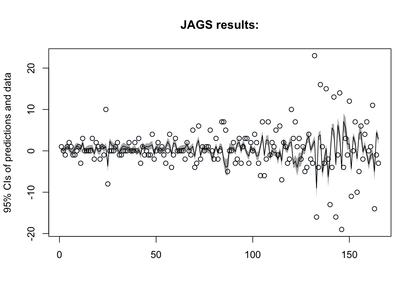
Here we see a graphical representation of model fit. The solid line indicates the median posterior draw, while the grey band shows the 95% credible interval at each time point. The points shown are the observed data points. Clearly, the model it too simple to capture the variability in the first difference.
| mean | sd | 2.5% | 25% | 50% | 75% | 97.5% | Rhat | n.eff | |
|---|---|---|---|---|---|---|---|---|---|
| mu | 0.39 | 0.21 | -0.04 | 0.25 | 0.39 | 0.52 | 0.81 | 1 | 13000 |
| phi | -0.46 | 0.07 | -0.59 | -0.51 | -0.46 | -0.41 | -0.30 | 1 | 15000 |
We see that the median estimate of \(\mu\) is 0.41 which makes sense. The ‘true’ data is increasing (as we previously saw) so the difference must have a positive mean. What is interesting is the estimates for the \(\phi\) estimate (median: -0.47, 95% Credible Interval: -0.61, -0.32). This suggests when we experience a deviation above the mean difference, we are likely to experience a following deviation below the mean difference.
While potentially marginally insightful we will move on to one of the most utilized time series models of all time.
Autoregressive Model AKA AR(1)
The auto regressive model is a classic time series model by which the models current value is a function of its previous value(s). The AR(1) model takes only into account the previous time’s value to model the current (or future) value.
Autoregressive (first order) model:
\(E(y_t) = \mu + y_{t-1} \phi + e_{t}\)
Note: AR(k) models don’t necessarily need to be stationary, making this a great fit for some real world data with non-constant mean.
We can specify this in JAGS as such:
ar1.model <- function(){
                mu ~ dnorm(0, 0.01);
                tau.pro ~ dgamma(0.001,0.001);
                sd.pro <- 1/sqrt(tau.pro);
                phi ~ dnorm(0, 1);
                predY[1] <- Y[1];
                for(i in 2:N) {
                        predY[i] <- mu + phi * Y[i-1];
                        Y[i] ~ dnorm(predY[i], tau.pro);
                }
}
ar1.data = list("Y"=chip_dat$hits,"N"=(N+1)) # n+1 because
                                        # the difference scores
                                        # have one less element
ar1.params=c("sd.pro","predY","mu","phi")
ar1.mcmc = jags(ar1.data, parameters.to.save=ar1.params,
                model.file=ar1.model,
                n.chains = 3,
                n.burnin=5000, n.thin=1,
                n.iter=10000, DIC=TRUE)
## Compiling model graph
## Resolving undeclared variables
## Allocating nodes
## Graph information:
## Observed stochastic nodes: 165
## Unobserved stochastic nodes: 3
## Total graph size: 310
##
## Initializing modelAR(1) Results
Lets checkout the plot:
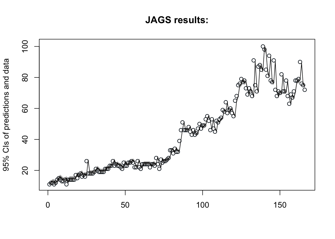
Now what are the estimates for our parameters?
| mean | sd | 2.5% | 25% | 50% | 75% | 97.5% | Rhat | n.eff | |
|---|---|---|---|---|---|---|---|---|---|
| mu | 1.37 | 0.82 | -0.24 | 0.82 | 1.37 | 1.92 | 2.96 | 1 | 15000 |
| phi | 0.98 | 0.02 | 0.94 | 0.97 | 0.98 | 0.99 | 1.01 | 1 | 10000 |
A natural extension of this model is the second degree autoregressive model - AR(2) which incorporates each elements previous two measurements, specified as such \(E(y_t) = \mu + y_{t-1} \phi_1 + y_{t-2} \phi_2 + e_{t}\)
So now that we’ve fit several models, we can compare them based on deviance information criterion (DIC).
The intercept model produced a DIC of 1022.6, while the autocorrelated error model and AR(1) produced DIC measures of 986.3 and 1054.4 respectively. An AR(2) model was also fit with a DIC greater than the AR(1). At first glance this may be surprising since a low DIC suggests a greater fit, we might be tempted to say that the autocorrelated error term has the greatest fit of all the models, however, the data utilized is not the same, and thus these models should not be compared based on DIC alone. After examining several other metrics into account, and taking into consideration the interpretability of each model, the AR(1) model is most appropriate, and we will use it to forecast interest in chipotle.
(Note: If we were to use the difference data for all models, the AR(1) would show a much lower DIC than any of the other models)
Forecasting Chipotle Sales
Predictions in JAGS are fairly easy, in the data we provide JAGS, we simply specify ‘future’ values as ‘NA’, and JAGS predicts them for us by continuing the MCMC chain. We can take these thousands of estimates and generate credible intervals and median estimates.
ar1.data.20 = list("Y"=c(chip_dat$hits,rep(NA,20)),"N"=N+20)
ar1.mcmc.20 = jags(ar1.data.20, parameters.to.save=ar1.params,
                  model.file=ar1.model, n.chains = 3, n.burnin=5000, n.thin=1,
                  n.iter=10000, DIC=TRUE)
## Compiling model graph
## Resolving undeclared variables
## Allocating nodes
## Graph information:
## Observed stochastic nodes: 165
## Unobserved stochastic nodes: 22
## Total graph size: 361
##
## Initializing modelNow, lets see what this looks like.
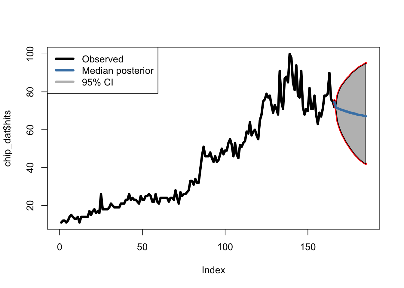
Our AR(1) model is predicting a decrease in chipotle interest in the coming 20 days - Let’s see if this holds!
What’s next?
While this was a lot of fun, there are much better models we can and should be using (some of which just simply didn’t make it to this post). Primarily moving average (MA), auto regressive integrated moving average (ARIMA), and state space models which are common to model real world data. In addition, it would be great to include covariates such as wages, sentiment analyses, and food prices, include seasonality, and incorporate hierarchical aspect given that we can extract location data as well.
In the meantime, lets see how well this model performs.
Feel free to comment or email with any questions!
Useful links / Resources used
- Anglim, Jeromy. Rjags, and Bayesian Modelling. http://jeromyanglim.blogspot.com/2012/04/getting-started-with-jags-rjags-and.html
- Hamilton, J. D. (1994). Time series analysis (Vol. 2). Princeton: Princeton university press.
- Holmes, Elizabeth. (2017). Introduction to Bayesian Time-Series Analysis using JAGS, University of Wisconson
- Metcalfe, A. V., & Cowpertwait, P. S. (2009). Introductory time series with R.