Beyond %>%, Alternative Pipes in R

Standard pipe: %>%

So, here we will do a short run through of the basic piping operator (%>%) for those new to the concept, and discuss some of other pipes that could be useful to experienced useRs. These pipes have a history of being introduced alongside the dplyr package, which together makes for some incredibly powerful, yet concise code (so powerful, during a technical job interview I was asked to stop using dplyr/pipes…).

The standard pipe takes the object to its left, and passes it as the first argument in the function to the right. When reading code, we can then read the pipe operator simply as: ‘then’.

library(datasets)
library(dplyr)
library(magrittr)
trees %>%
        dplyr::filter(Girth > 9) %>%
        dplyr::select(Height, Volume) %>%
        summary()

##      Height          Volume     
##  Min.   :64.00   Min.   :15.60  
##  1st Qu.:74.00   1st Qu.:20.73  
##  Median :77.50   Median :25.30  
##  Mean   :77.07   Mean   :32.30  
##  3rd Qu.:80.25   3rd Qu.:39.38  
##  Max.   :87.00   Max.   :77.00

This can be read as “Take the trees data set, then show only the trees with girth greater than 9, then select the height and volume of those trees, then compute summary statistics on those two variables”.

Without pipes we’d use:

# complete base R way:
summary(trees[trees$Girth > 9, 2:3])

##      Height          Volume     
##  Min.   :64.00   Min.   :15.60  
##  1st Qu.:74.00   1st Qu.:20.73  
##  Median :77.50   Median :25.30  
##  Mean   :77.07   Mean   :32.30  
##  3rd Qu.:80.25   3rd Qu.:39.38  
##  Max.   :87.00   Max.   :77.00

# or

# using dplyr
trees_of_interest <- dplyr::filter(trees, Girth > 9)
vars_of_interest <- dplyr::select(trees_of_interest, Height, Volume)
summary(vars_of_interest)

##      Height          Volume     
##  Min.   :64.00   Min.   :15.60  
##  1st Qu.:74.00   1st Qu.:20.73  
##  Median :77.50   Median :25.30  
##  Mean   :77.07   Mean   :32.30  
##  3rd Qu.:80.25   3rd Qu.:39.38  
##  Max.   :87.00   Max.   :77.00

Very quickly we can identify the benefits here, readability. With %>% we can read the data munging process from left to right, just like English. Compare this with the ‘base R’ approach in the second chunk - have to read as a mix of left to right with functions being called on parsed objects - quite a mess. Even using dplyr is not enough to make this process readable, we’ve just created two additional data frames just to compute these summary statistics (which, not to mention, could be computationally intense in bigger datasets).

Tree pipe: %T>%

The tree pipe is very similar to the standard pipe, however, it returns the left input instead of the operated value. Check out the difference below:

1:10 %>%
        mean()

## [1] 5.5

1:10 %T>%
        mean()

##  [1]  1  2  3  4  5  6  7  8  9 10

You might be wondering why this is useful, which is fair. This operator works very well plotting data mid ‘pipeline’ as well as in some other, more niche areas.

For example, say we are wrangling data, want to plot it, but also would like to visualize it:

library(datasets)
mtcars %>%
        dplyr::group_by(cyl) %>%
        dplyr::summarise(mean_hp = mean(hp)) %T>%
        plot(main = "Horsepower by cylinders - mtcars edition",
             xlab = "cylinders", ylab = "horse power",
             type = "l", lwd = 3, col = "steelblue")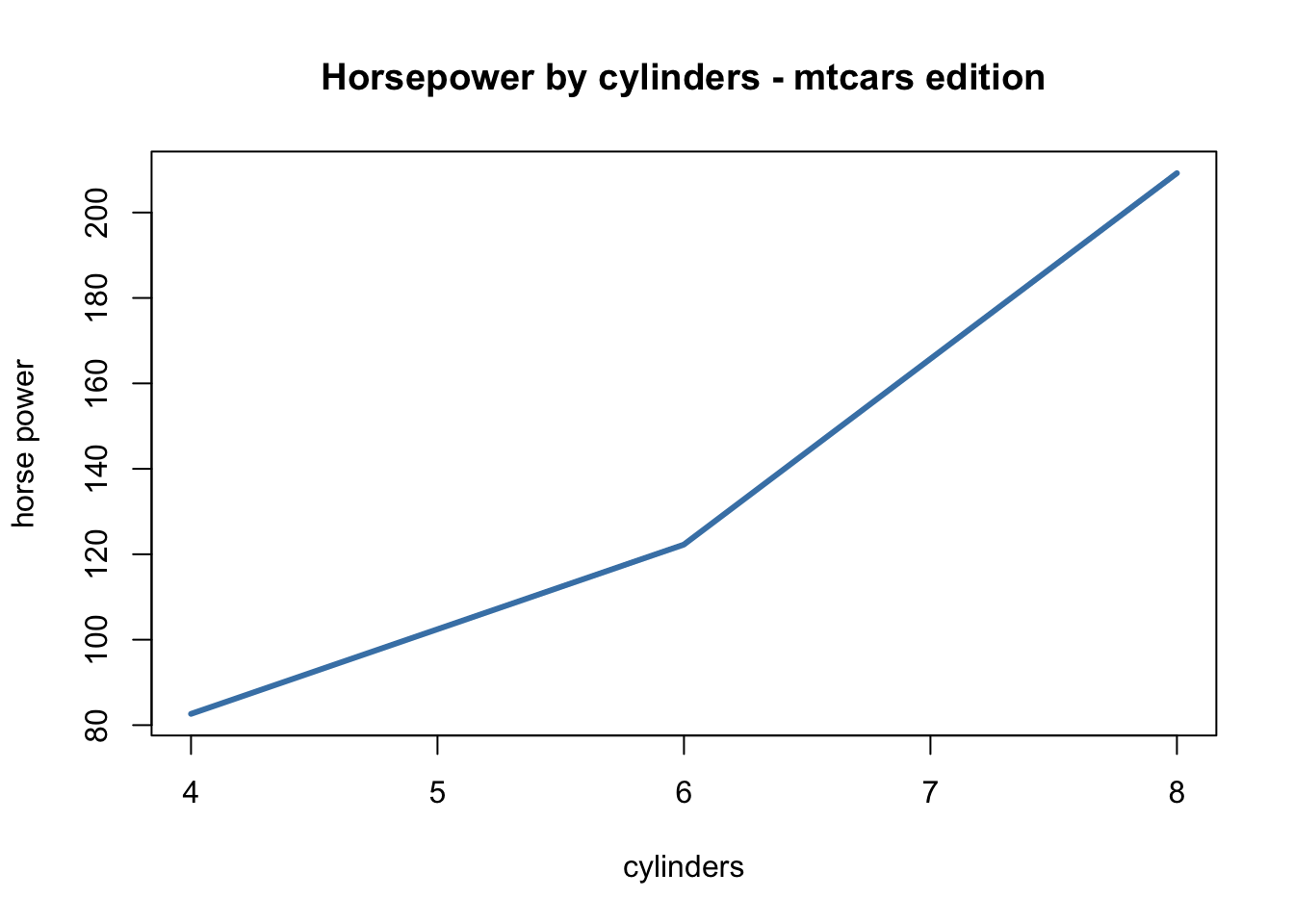

## # A tibble: 3 x 2
##     cyl   mean_hp
##   <dbl>     <dbl>
## 1     4  82.63636
## 2     6 122.28571
## 3     8 209.21429

Here we were able to return a nice plot as well as a data matrix without rewriting / copy & pasting code.

Exposition pipe: %$%

Admittedly, this is not a pipe operator I have used often (read: at all), but it is featured in the package. Essentially %$% is a ‘pipe friendly’ way to pull objects from a data frame, similarly to the base R method of using $ to extract a single element (column) from an object (data frame, typically).

Thus, writing this code to plot a box plot from the horsepower (hp) vector of the mtcars data could be written like this:

boxplot(mtcars$hp)

or, using the exposition pipe, like the following:

mtcars %$%
  boxplot(hp)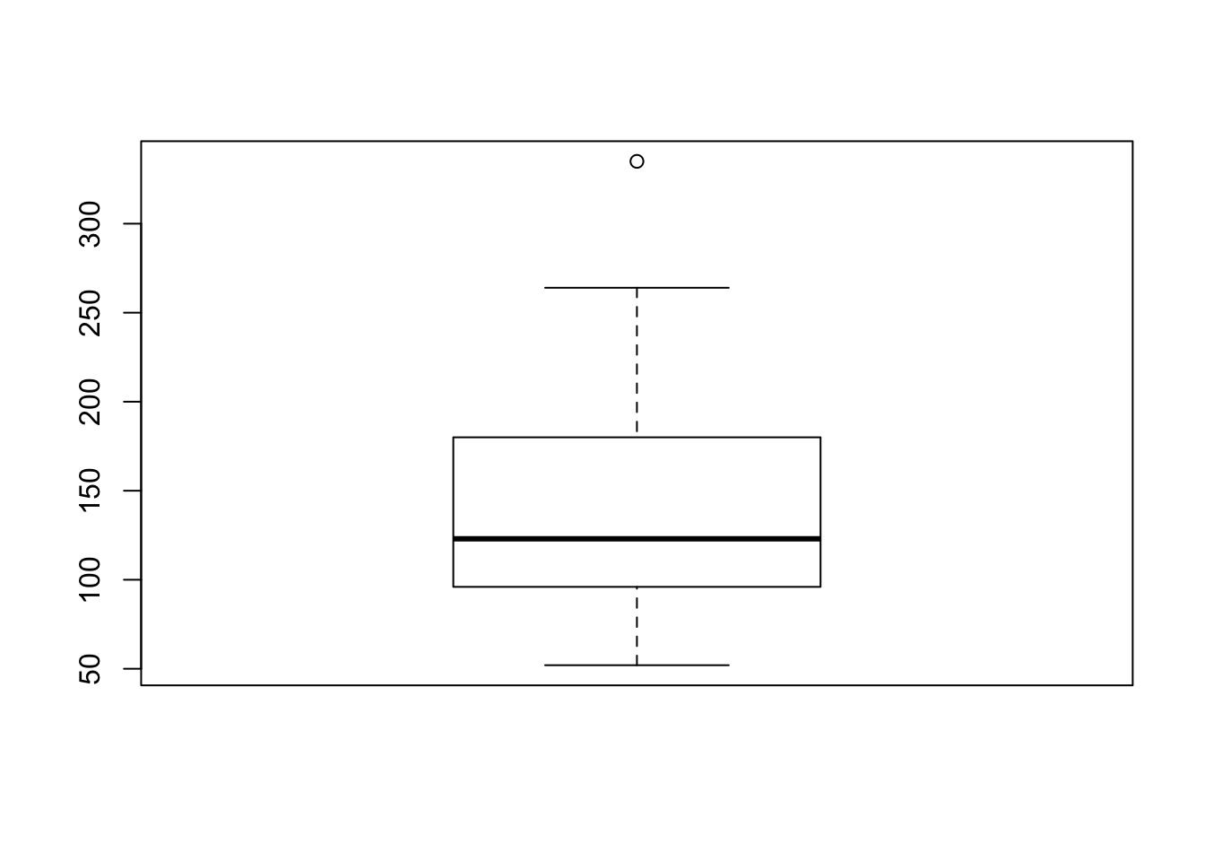

Without knowing the exposition pipe I may have written the same code as:

mtcars %>%
        dplyr::select(hp) %>%
        boxplot()

This results in the exact same output as the previous two chunks, but is one line longer than the exposition example - I will be sure to include it in my toolbox!

compound assignment pipe: %<>%

Here it is important to note that there are many different philosophies regarding nearly all aspects of data management, particularly when it comes to overwriting your data. While there are certain circumstances where overwriting may be ok, it is always important to be careful! The compound assignment pipe rewrites the left hand object with the output of the function to the right.

In practice:

set.seed(100)

x <- rnorm(100)
x %<>% round() %>% median()
x

## [1] 0

What happened here? We defined x as a string of 100 random standard normals, then reassigned x as the median rounded value. This could save a little bit of typing as I typically see the following:

set.seed(100)

x <- rnorm(100)
x <- x %>% round() %>% median()
x

## [1] 0

In short:

Pipes are not absolutely required for any particular analysis, but can drastically improve readability and reduce the number of lines needed (two sometimes competing birds with one stone here!). Once you have mastered the standard pipe (%>%) you should spend some time exploring and utilizing the others, as they function well in different yet common situations. I for one am going to spend some more time with the exposition pipe which can help shave a line of code when selecting a single column from a data frame.

Follow the discussion

Follow the discussion on reddit or below!

Let me know if you have any questions or comments!