Q: What does modeling the number of people buying gelato in Venice using cultural data and environmental attributes have in common with assessing which measures of reading speed are most related to glaucoma propensity?
A: A strong need for variable selection.
Whenever we consider estimating the relationship between two variables, say \(x\) and \(y\), we need to contemplate what other factors may be associated with those of interest and whether or not to include them in our model. In addition, sometimes, we may have many variables at our disposal, and need to narrow down which ones provide substantial relevant information in order explain the data in a simple way, avoid overfitting, or reduce costs [in terms of both data collection and, potentially storing/analyzing]. This problem of covariate selection can be tough - how can we include relevant and otherwise important variables in our models while excluding those with unsubstantial or happenstantial relationships? Here, we will look at a common mistake - the use of step-wise-backward selection in regression analysis.
Suppose we have data concerning \(y\) and a handful of predictors, \(x_i\)’s. Say we are interested in assessing the relationship between these variables, \(x_i\) and \(y\), but aren’t sure which variables to include. Backward selection is sometimes employed to isolate only the relevant variables by removing seemingly irrelevant covariates in a one-at-a-time process. The general protocol is to fit a ‘full model’ using all available covariates (all \(x_i\)’s), and then remove the \(x_i\) with the weakest relationship one at a time until some stopping criteria is reached:
Backward Step-wise selection/elimination algorithm [linear regression case]
- Fit a full model using all \(N\) \(x_i\)’s
- \(\hat{y} = \beta_0 + \beta_1 x_1 + ... + \beta_N x_N\)
- Remove \(x_i\) with the weakest relationship and refit the model.
- Usually the least significant variable, if one exists, is dropped, and the model refit.
- \(\hat{y} = \beta_0 + \beta_1 x_1 + \beta_{i-1} x_{i-1} + \beta_{i+1} x_{i+1} + ... + \beta_N x_N\)
- Repeat 2 until a stopping criteria is reached.
- Could be when all remaining coefficient p-values are less than the predefined \(\alpha\) value [say, 0.05], or there is only one coefficient remaining.
P-values and their properties
In order to see and understand why step-wise backward selection may not be an ideal method of covariate selection, we must understand a bit more about p-values. We will accomplish this be examining the distribution of p-values under the null hypothesis where \(x\) is independent of \(y\).
First, let’s set our seed and load some dependencies.
# R 3.3.2
library("dplyr")
library("broom")
set.seed(123)
Let’s say we are interested in understanding the relationship between \(x_1\) and \(y\), which under the null hypothesis, \(x_1\) and \(y\) are independent.
Under the null, what would be expect?
Well, lets set our significance/\(\alpha\)-level to 0.05. By definition of \(\alpha\)-level we know that approximately 5% of our results would be significant despite there being no actual relationship present. Furthermore, because there is no real relationship, we would also expect the resulting p-values to be uniform on (0,1).
Let’s take a look at 1,000 simulated situations where the linear relationship between \(x_1\) and \(y\) is compared where both variables are actually independent of one another - I’ll using dplyr for better readability:
x <- vector()
sim1 <- 1000
# lets run this simulation 10,000 times
for (i in 1:sim1){

        data_set <- data.frame(rnorm(1000), rnorm(1000))

        colnames(data_set) <- c("y","x")

        # lets fit our linear model
        p_val <- lm(y ~ x, data = data_set) %>%

        # then lets extract our 'tidy' output
                broom::tidy() %>%

        # then we will remove the intercept coefficient
                dplyr::slice(-1) %>%

        # then we will select select our p-values
                dplyr::select(p.value) #%>%

        # storing our generated p-value in a list of p-values
        x <- append(x, p_val)

}

# storing our list of p-values as a vector for easier plotting etc.
x <- as.numeric(x)

# looking at our results
hist(x,
     col = "steelblue",
     main = "Distribution of p-values",
     # sub = "test",
     xlab = "P-value",
     ylab = "Count")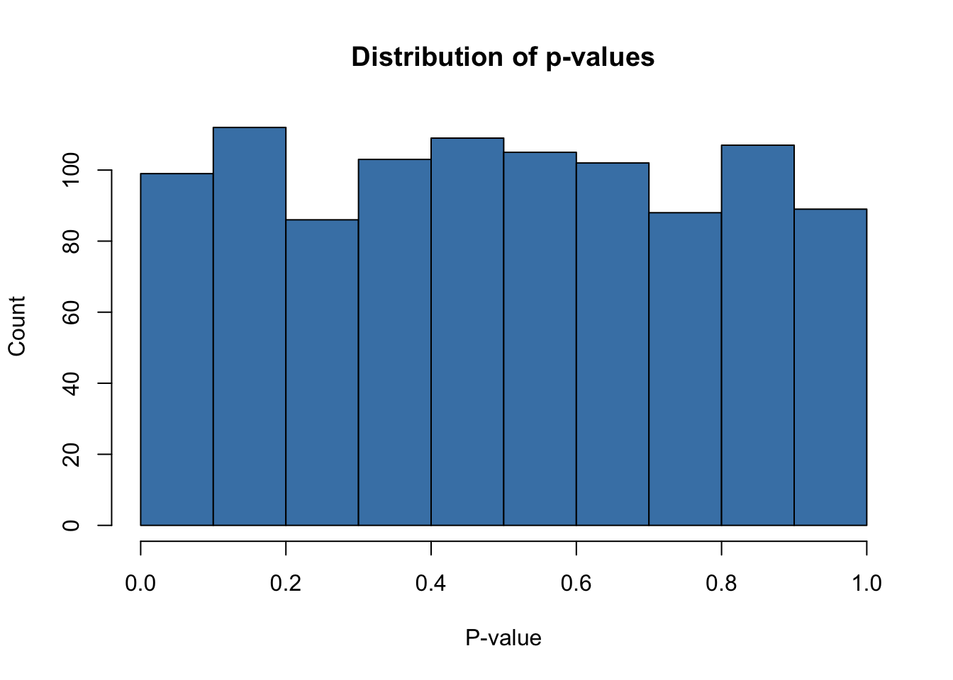
Distribution of p-values in our null, simple linear regression case. Note - the distribution of p-values is what we’d expect, seemingly uniform distribution with \(49\) [\(4.9\) %] of our simulated examples reaching sub-\(\alpha\) level significance. The take away here is that the percentage of false positives [our realized type I error rate] is very close to our theoretical estimate of 5%, our A priori Type I error rate - exactly what we would hope.
Now that we understand some of the behavior of p-values, let’s take a look at backward selection using 2 variables.
Backward Selection
Our Backward Step-wise selection/elimination algorithm
- Fit a full model using \(x_1\) & \(x_2\).
- \(\hat{y} = \beta_0 + \beta_1 x_1 + \beta_2 x_2\)
- If at least \(\beta_1\) or \(\beta_2\) is non significant, remove \(x_i\) with the weakest relationship and refit the model otherwise move to 3.
- $ = _0 + _i x_i where _i is more significant and _j is not.
- Stop removing covariates when either both \(\beta_1\) & \(\beta_2\) are significant, or there is only one variable remaining.
We would expect that, under the null hypothesis: both \(x_1\) and \(x_2\) are independent of \(y\) and \(x_1\) and \(x_2\) are independent of themselves, there would be:
- \(0.005^2 \times 1000 =0.025\) simulated runs where both coefficients are significant.
- \((0.05 + 0.05 - 2 \times 0.05^2) * 10000 = 95\) simulated runs where one coefficient is significant.
x2 <- vector()

double_sig <- 0

# lets simulate this situation 10000 times.
sim2_num <- 1000
for (i in 1:sim2_num){

        # creating testing data
        data_set <- data.frame(rnorm(1000),
                rnorm(1000),
                rnorm(1000)
                )

        colnames(data_set) <- c("y", "x1", "x2")

        #fitting lm
        p_vals <- lm(y ~ x1 + x2, data = data_set) %>%

        # then obtaining tidy output
                broom::tidy() %>%

        # then removing intercept coef
                dplyr::slice(-1) %>%

        # then selecting pvalues
                dplyr::select(term, p.value)

        # checking stopping criteria
        # IF both at least one coefficients is not significant
        # then we remove the coefficient with a higher p-value
        # and re-run the regression

        if (sum(p_vals$p.value > 0.05) >= 1) {
                var_keep <- which.min(p_vals$p.value) + 1
                data_set <- data_set %>%
                        dplyr::select(c(1,var_keep))

                p_vals <- lm(y ~ ., data = data_set) %>%
                        broom::tidy() %>%
                        dplyr::slice(-1) %>%
                        dplyr::select(p.value) %>%
                        as.numeric()

                x2 <- append(x2, p_vals)

        # otherwise, we will record that both coefficients were significant
        } else {
                double_sig <- double_sig + 1
        }
}
Out of the 1000 simulations, 2 [0.2%] were significant at both coefficients. These results were right on par with our theoretical estimations made prior to the simulation.
Similarly however, the number of simulations with exactly one coefficient appearing as significant was 115 [11.5%].
Here lies the important problem:
If you were to conduct this backward selection in the same way and report one of these regression results, and call all coefficients with a p-value below 0.05 as significant, your true false positive rate would actually be much higher. As we saw in this analysis, despite there being no real relationship between either \(x\) or \(y\), we recorded that of the 1000 simulated regressions 998 utilized the backward selection algorithm to drop the least significant coefficient. If a researcher/scientist/statistician reported such a regression, their probability of a type 1 error would be about 11.7%, despite being at an \(\alpha\) level of 0.05, suggesting false confidence in the results as an improper . This severe Type I error rate inflation could be dangerous, signaling extraneous relationships as real, and leading researchers in the wrong direction.
hist(x2,
     col = "steelblue",
     main = "Distribution of p-values",
     xlab = "P-values")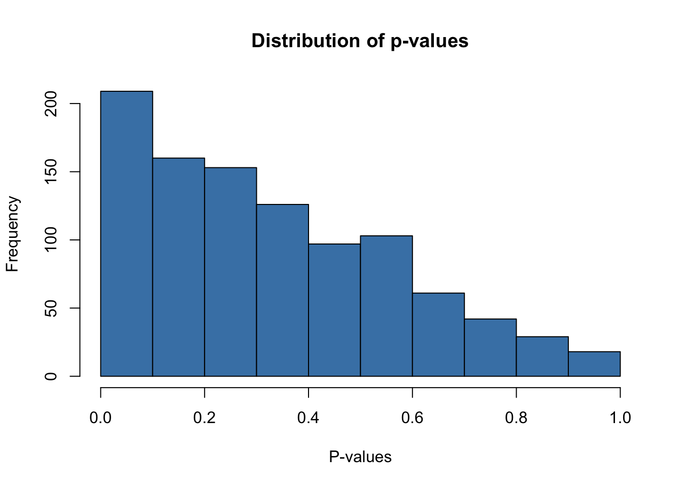
Distribution of p-values excluding the 2 observations where both observations were significant is non-uniform. Clearly we can see very strong skewness towards small p-values despite the absence of any relationship between \(x_1\) or \(x_2\) and \(y\) whatsoever.
Other Options and Takeaways
As we saw here, even a small alteration to our methodologies can have striking effects on our type I error rates, and in turn our results and interpretations. It is important when doing any sort of selection method to consider how this type I error rate [which is really one of the most important concepts of hypothesis testing] may be changing, and report it. Model and covariate selection are tricky concepts, partly for the same reason outlined above. Even some ‘robust’ methodologies such as the LASSO can be tainted with bias [although in a bit different form]. The best defense to these issues can be to understand what biases may be occurring and accounting for them. For instance, it still may be possible to utilize backward selection by using a p-value correction method.
Links
- Ingo’s notes on Variable Selection
- Problems with the LASSO
- This analyis